로지스틱 (2) – 손실함수의 비교 // 깊은신경망 (1) – 로지스틱의 한계, DNN을 이용한 해결, DNN으로 해결가능한 다양한 예제
강의영상
https://youtube.com/playlist?list=PLQqh36zP38-zE7DY6FYyM9eVy0HTIkwNB
imports
시각화를 위한 준비함수들
준비1 loss_fn을 plot하는 함수
def plot_loss(loss_fn,ax=None):
if ax==None:
fig = plt.figure()
ax=fig.add_subplot(1,1,1,projection='3d')
ax.elev=15;ax.azim=75
w0hat,w1hat =torch.meshgrid(torch.arange(-10,3,0.15),torch.arange(-1,10,0.15),indexing='ij')
w0hat = w0hat.reshape(-1)
w1hat = w1hat.reshape(-1)
def l(w0hat,w1hat):
yhat = torch.exp(w0hat+w1hat*x)/(1+torch.exp(w0hat+w1hat*x))
return loss_fn(yhat,y)
loss = list(map(l,w0hat,w1hat))
ax.scatter(w0hat,w1hat,loss,s=0.1,alpha=0.2)
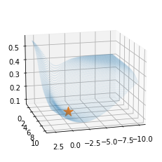
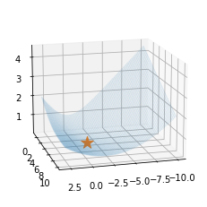
ax.scatter(-1,5,l(-1,5),s=200,marker='*') # 실제로 -1,5에서 최소값을 가지는건 아님.. - \(y_i \sim Ber(\pi_i),\quad\) where \(\pi_i = \frac{\exp(-1+5x_i)}{1+\exp(-1+5x_i)}\) 에서 생성된 데이터 한정하여 손실함수가 그려지게 되어있음.
준비2: for문 대신 돌려주고 epoch마다 필요한 정보를 기록하는 함수
def learn_and_record(net, loss_fn, optimizr):
    yhat_history = []
    loss_history = []
    what_history = []

    for epoc in range(1000):
        ## step1
        yhat = net(x)
        ## step2
        loss = loss_fn(yhat,y)
        ## step3
        loss.backward()
        ## step4
        optimizr.step()
        optimizr.zero_grad()

        ## record
        if epoc % 20 ==0:
            yhat_history.append(yhat.reshape(-1).data.tolist())
            loss_history.append(loss.item())
            what_history.append([net[0].bias.data.item(), net[0].weight.data.item()])
return yhat_history, loss_history, what_history- 20에폭마다 yhat, loss, what을 기록
준비3: 애니메이션을 만들어주는 함수
def show_lrpr2(net,loss_fn,optimizr,suptitle=''):
    yhat_history,loss_history,what_history = learn_and_record(net,loss_fn,optimizr)

    fig = plt.figure(figsize=(7,2.5))
    ax1 = fig.add_subplot(1, 2, 1)
    ax2 = fig.add_subplot(1, 2, 2, projection='3d')
    ax1.set_xticks([]);ax1.set_yticks([])
    ax2.set_xticks([]);ax2.set_yticks([]);ax2.set_zticks([])
    ax2.elev = 15; ax2.azim = 75

    ## ax1: 왼쪽그림
    ax1.plot(x,v,'--')
    ax1.scatter(x,y,alpha=0.05)
    line, = ax1.plot(x,yhat_history[0],'--')
    plot_loss(loss_fn,ax2)
    fig.suptitle(suptitle)
    fig.tight_layout()

    def animate(epoc):
        line.set_ydata(yhat_history[epoc])
        ax2.scatter(np.array(what_history)[epoc,0],np.array(what_history)[epoc,1],loss_history[epoc],color='grey')
        return line

    ani = animation.FuncAnimation(fig, animate, frames=30)
    plt.close()
return ani- 준비1에서 그려진 loss 함수위에, 준비2의 정보를 조합하여 애니메이션을 만들어주는 함수
Logistic intro (review + \(\alpha\))
- 모델: \(x\)가 커질수록 \(y=1\)이 잘나오는 모형은 아래와 같이 설계할 수 있음 <— 외우세요!!!
$y_i Ber(_i),$ where \(\pi_i = \frac{\exp(w_0+w_1x_i)}{1+\exp(w_0+w_1x_i)}\)
\(\hat{y}_i= \frac{\exp(\hat{w}_0+\hat{w}_1x_i)}{1+\exp(\hat{w}_0+\hat{w}_1x_i)}=\frac{1}{1+\exp(-\hat{w}_0-\hat{w}_1x_i)}\)
\(loss= - \sum_{i=1}^{n} \big(y_i\log(\hat{y}_i)+(1-y_i)\log(1-\hat{y}_i)\big)\) <— 외우세요!!
- toy example
- step1: yhat을 만들기
(방법1)
torch.manual_seed(43052)
l1=torch.nn.Linear(1,1)
a1=torch.nn.Sigmoid()
yhat= a1(l1(x)) # yhat=net(x) 라고 쓰고싶어 사실
yhat
tensor([[0.3775],
[0.3774],
[0.3773],
...,
[0.2327],
[0.2327],
[0.2326]], grad_fn=<SigmoidBackward0>)(방법2)
\(x \overset{l1}{\to} u \overset{a1}{\to} v = \hat{y}\)
\(x \overset{net}{\to} \hat{y}\)
torch.manual_seed(43052)
l1=torch.nn.Linear(1,1)
a1=torch.nn.Sigmoid()
net = torch.nn.Sequential(l1,a1)
yhat= net(x) # a1(l1(x))
yhat
tensor([[0.3775],
[0.3774],
[0.3773],
...,
[0.2327],
[0.2327],
[0.2326]], grad_fn=<SigmoidBackward0>)(방법3)
torch.manual_seed(43052)
net = torch.nn.Sequential(
    torch.nn.Linear(1,1),
    torch.nn.Sigmoid()
)
yhat= net(x) # a1(l1(x))
yhat
tensor([[0.3775],
[0.3774],
[0.3773],
...,
[0.2327],
[0.2327],
[0.2326]], grad_fn=<SigmoidBackward0>)- step2
(방법1)
(방법2)
- step 1~4

로지스틱–BCEloss
- step 1~4
- 왜?? “linear -> sigmoid” 로 yhat을 구하고 BCELoss로 loss를 계산하면 그 모양이 convex하게 되므로
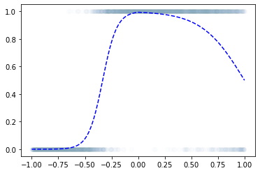
시각화1: MSE, 좋은초기값
시각화2: MSE, 나쁜초기값
시각화3: BCE, 좋은초기값
시각화4: BCE, 나쁜초기값
로지스틱–Adam (국민옵티마이저)
- Adam은 SGD에 비하여 2가지 면에서 개선점이 있음. 1. 몰라도 됩니다.. 2. 가속도의 개념
시각화1: MSE, 좋은초기값 –> 이걸 아담으로!
시각화2: MSE, 나쁜초기값 –> 이걸 아담으로! (혼자해봐요..)
시각화3: BCE, 좋은초기값 –> 이걸 아담으로! (혼자해봐요..)
시각화4: BCE, 나쁜초기값 –> 이걸 아담으로! (혼자해봐요..)
깊은신경망–로지스틱 회귀의 한계
신문기사 (데이터의 모티브)
중소·지방 기업 “뽑아봤자 그만두니까”
중소기업 관계자들은 고스펙 지원자를 꺼리는 이유로 높은 퇴직률을 꼽는다. 여건이 좋은 대기업으로 이직하거나 회사를 관두는 경우가 많다는 하소연이다. 고용정보원이 지난 3일 공개한 자료에 따르면 중소기업 청년취업자 가운데 49.5%가 2년 내에 회사를 그만두는 것으로 나타났다.
중소 IT업체 관계자는 “기업 입장에서 가장 뼈아픈 게 신입사원이 그만둬서 새로 뽑는 일”이라며 “명문대 나온 스펙 좋은 지원자를 뽑아놔도 1년을 채우지 않고 그만두는 사원이 대부분이라 우리도 눈을 낮춰 사람을 뽑는다”고 말했다.
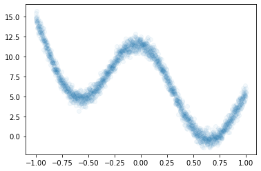
가짜데이터
- 위의 기사를 모티브로 한 데이터
df=pd.read_csv('https://raw.githubusercontent.com/guebin/DL2022/master/posts/2022-10-04-dnnex0.csv')
df| x | underlying | y | |
|---|---|---|---|
| 0 | -1.000000 | 0.000045 | 0.0 |
| 1 | -0.998999 | 0.000046 | 0.0 |
| 2 | -0.997999 | 0.000047 | 0.0 |
| 3 | -0.996998 | 0.000047 | 0.0 |
| 4 | -0.995998 | 0.000048 | 0.0 |
| ... | ... | ... | ... |
| 1995 | 0.995998 | 0.505002 | 0.0 |
| 1996 | 0.996998 | 0.503752 | 0.0 |
| 1997 | 0.997999 | 0.502501 | 0.0 |
| 1998 | 0.998999 | 0.501251 | 1.0 |
| 1999 | 1.000000 | 0.500000 | 1.0 |
2000 rows × 3 columns
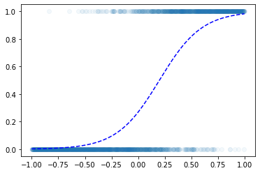
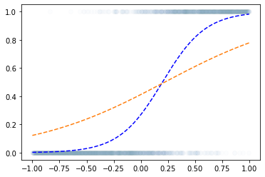
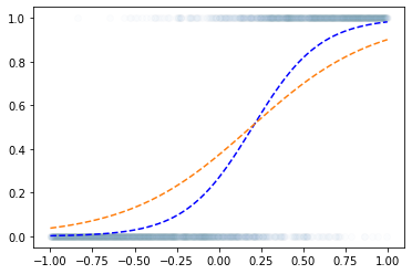
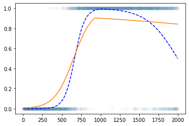
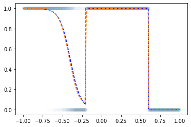
로지스틱 회귀로 적합
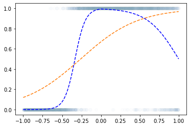
- 이거는 epoc=60억해도 주황색 점선은 절대 파란색 점선이 될 수 없다.
해결책
- sigmoid를 취하기 전의 상태가 꺽인 그래프여야 한다.
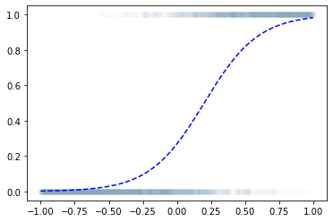
깊은신경망–DNN을 이용한 해결
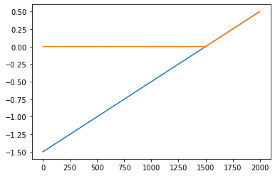
- 목표: 아래와 같은 벡터 \({\boldsymbol u}\)를 만들어보자.
\({\boldsymbol u} = [u_1,u_2,\dots,u_{2000}], \quad u_i = \begin{cases} 9x_i +4.5& x_i <0 \\ -4.5x_i + 4.5& x_i >0 \end{cases}\)
꺽인 그래프를 만드는 방법1
꺽인 그래프를 만드는 방법2
- 전략: 선형변환 \(\to\) ReLU \(\to\) 선형변환
(예비학습) ReLU 함수란?
\(ReLU(x) = \max(0,x)\)
(선형변환1)

(렐루)
plt.plot(x,alpha=0.5,color='C0')
plt.plot(-x,alpha=0.5,color='C1')
plt.plot(rlu(x),color='C0')
plt.plot(rlu(-x),color='C1')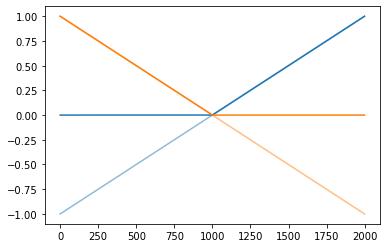
(선형변환2)
plt.plot(x,alpha=0.2,color='C0')
plt.plot(-x,alpha=0.2,color='C1')
plt.plot(rlu(x),color='C0',alpha=0.2)
plt.plot(rlu(-x),color='C1',alpha=0.2)
plt.plot(-4.5*rlu(x)+-9*rlu(-x)+4.5,color='C2')
#plt.plot(u)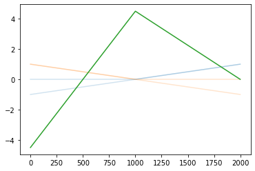
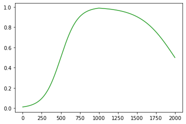
(시그모이드)
정리하면!
fig = plt.figure(figsize=(8, 4))
spec = fig.add_gridspec(4, 4)
ax1 = fig.add_subplot(spec[:2,0]); ax1.set_title('x'); ax1.plot(x,'--',color='C0')
ax2 = fig.add_subplot(spec[2:,0]); ax2.set_title('-x'); ax2.plot(-x,'--',color='C1')
ax3 = fig.add_subplot(spec[:2,1]); ax3.set_title('relu(x)'); ax3.plot(rlu(x),'--',color='C0')
ax4 = fig.add_subplot(spec[2:,1]); ax4.set_title('relu(-x)'); ax4.plot(rlu(-x),'--',color='C1')
ax5 = fig.add_subplot(spec[1:3,2]); ax5.set_title('u'); ax5.plot(-4.5*rlu(x)-9*rlu(-x)+4.5,'--',color='C2')
ax6 = fig.add_subplot(spec[1:3,3]); ax6.set_title('yhat'); ax6.plot(sig(-4.5*rlu(x)-9*rlu(-x)+4.5),'--',color='C2')
fig.tight_layout()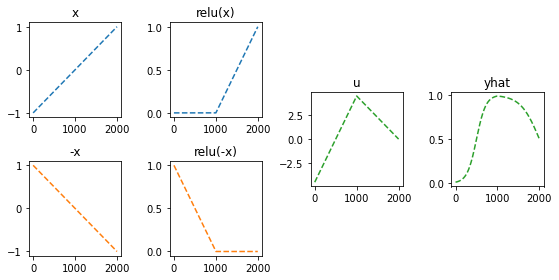
- 이런느낌으로 \(\hat{\boldsymbol y}\)을 만들면 된다.
torch.nn.Linear()를 이용한 꺽인 그래프 구현
- 구현
plt.plot(y,'o',alpha=0.02)
plt.plot(df.underlying,'--b')
#plt.plot(a2(l2(a1(l1(x)))).data)
plt.plot(net(x).data)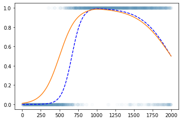
- 수식표현
(1) \({\bf X}=\begin{bmatrix} x_1 \\ \dots \\ x_n \end{bmatrix}\)
(2) \(l_1({\bf X})={\bf X}{\bf W}^{(1)}\overset{bc}{+} {\boldsymbol b}^{(1)}=\begin{bmatrix} x_1 & -x_1 \\ x_2 & -x_2 \\ \dots & \dots \\ x_n & -x_n\end{bmatrix}\)
- \({\bf W}^{(1)}=\begin{bmatrix} 1 & -1 \end{bmatrix}\)
- \({\boldsymbol b}^{(1)}=\begin{bmatrix} 0 & 0 \end{bmatrix}\)
(3) \((a_1\circ l_1)({\bf X})=\text{relu}\big({\bf X}{\bf W}^{(1)}\overset{bc}{+}{\boldsymbol b}^{(1)}\big)=\begin{bmatrix} \text{relu}(x_1) & \text{relu}(-x_1) \\ \text{relu}(x_2) & \text{relu}(-x_2) \\ \dots & \dots \\ \text{relu}(x_n) & \text{relu}(-x_n)\end{bmatrix}\)
(4) \((l_2 \circ a_1\circ l_1)({\bf X})=\text{relu}\big({\bf X}{\bf W}^{(1)}\overset{bc}{+}{\boldsymbol b}^{(1)}\big){\bf W}^{(2)}\overset{bc}{+}b^{(2)}\)
\(\quad=\begin{bmatrix} -4.5\times\text{relu}(x_1) -9.0 \times \text{relu}(-x_1) +4.5 \\ -4.5\times\text{relu}(x_2) -9.0 \times\text{relu}(-x_2) + 4.5 \\ \dots \\ -4.5\times \text{relu}(x_n) -9.0 \times\text{relu}(-x_n)+4.5 \end{bmatrix}\)
- \({\bf W}^{(2)}=\begin{bmatrix} -4.5 \\ -9 \end{bmatrix}\)
- \(b^{(2)}=4.5\)
(5) \(net({\bf X})=(a_2 \circ l_2 \circ a_1\circ l_1)({\bf X})=\text{sig}\Big(\text{relu}\big({\bf X}{\bf W}^{(1)}\overset{bc}{+}{\boldsymbol b}^{(1)}\big){\bf W}^{(2)}\overset{bc}{+}b^{(2)}\Big)\)
\(\quad =\begin{bmatrix} \text{sig}\Big(-4.5\times\text{relu}(x_1) -9.0 \times \text{relu}(-x_1) +4.5\Big) \\ \text{sig}\Big(-4.5\times\text{relu}(x_2) -9.0 \times\text{relu}(-x_2) + 4.5 \Big)\\ \dots \\ \text{sig}\Big(-4.5\times \text{relu}(x_n) -9.0 \times\text{relu}(-x_n)+4.5 \Big)\end{bmatrix}\)
- 차원만 따지자
\(\underset{(n,1)}{\bf X} \overset{l_1}{\to} \underset{(n,2)}{\boldsymbol u^{(1)}} \overset{a_1}{\to} \underset{(n,2)}{\boldsymbol v^{(1)}} \overset{l_2}{\to} \underset{(n,1)}{\boldsymbol u^{(2)}} \overset{a_2}{\to} \underset{(n,1)}{\boldsymbol v^{(2)}}=\underset{(n,1)}{\hat{\boldsymbol y}}\)
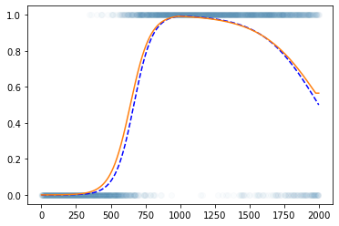
Step1 ~ Step4
- 추가로 3000번 더
깊은신경망–DNN으로 해결가능한 다양한 예제
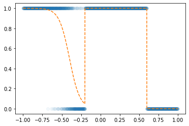
예제1
df = pd.read_csv('https://raw.githubusercontent.com/guebin/DL2022/master/posts/2022-10-04-dnnex1.csv')
df| x | underlying | y | |
|---|---|---|---|
| 0 | -1.000000 | 0.999877 | 1.0 |
| 1 | -0.998999 | 0.999875 | 1.0 |
| 2 | -0.997999 | 0.999873 | 1.0 |
| 3 | -0.996998 | 0.999871 | 1.0 |
| 4 | -0.995998 | 0.999869 | 1.0 |
| ... | ... | ... | ... |
| 1995 | 0.995998 | 0.000123 | 0.0 |
| 1996 | 0.996998 | 0.000123 | 0.0 |
| 1997 | 0.997999 | 0.000123 | 0.0 |
| 1998 | 0.998999 | 0.000123 | 0.0 |
| 1999 | 1.000000 | 0.000123 | 0.0 |
2000 rows × 3 columns
- 데이터정리
- for문을 돌리기 위한 준비
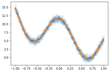
예제2
df = pd.read_csv('https://raw.githubusercontent.com/guebin/DL2022/master/posts/2022-10-04-dnnex2.csv')
df| x | underlying | y | |
|---|---|---|---|
| 0 | -1.000000 | 14.791438 | 14.486265 |
| 1 | -0.999000 | 14.756562 | 14.832600 |
| 2 | -0.997999 | 14.721663 | 15.473211 |
| 3 | -0.996999 | 14.686739 | 14.757734 |
| 4 | -0.995998 | 14.651794 | 15.042901 |
| ... | ... | ... | ... |
| 1995 | 0.995998 | 5.299511 | 5.511416 |
| 1996 | 0.996999 | 5.322140 | 6.022263 |
| 1997 | 0.997999 | 5.344736 | 4.989637 |
| 1998 | 0.999000 | 5.367299 | 5.575369 |
| 1999 | 1.000000 | 5.389829 | 5.466730 |
2000 rows × 3 columns
- 데이터준비
- for문 돌릴 준비
- step1~4
plt.plot(df.x,df.y,'o',alpha=0.05)
plt.plot(df.x,df.underlying,'--b')
plt.plot(x,net(x).data,'--',lw=5)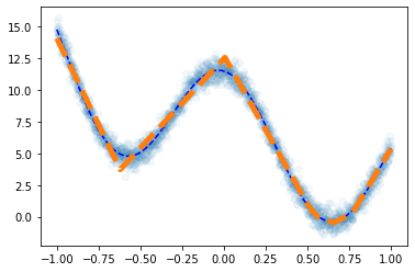
- for문 돌릴 준비
- step1~4
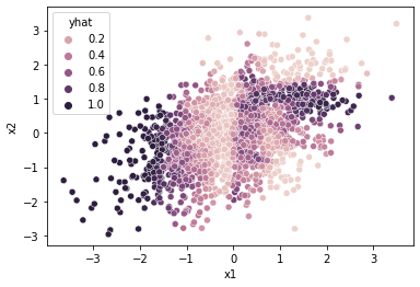
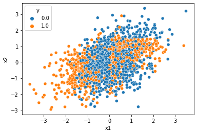
예제3
df = pd.read_csv('https://raw.githubusercontent.com/guebin/DL2022/master/posts/2022-10-04-dnnex3.csv')
df| x1 | x2 | y | |
|---|---|---|---|
| 0 | -0.874139 | 0.210035 | 0.0 |
| 1 | -1.143622 | -0.835728 | 1.0 |
| 2 | -0.383906 | -0.027954 | 0.0 |
| 3 | 2.131652 | 0.748879 | 1.0 |
| 4 | 2.411805 | 0.925588 | 1.0 |
| ... | ... | ... | ... |
| 1995 | -0.002797 | -0.040410 | 0.0 |
| 1996 | -1.003506 | 1.182736 | 0.0 |
| 1997 | 1.388121 | 0.079317 | 0.0 |
| 1998 | 0.080463 | 0.816024 | 1.0 |
| 1999 | -0.416859 | 0.067907 | 0.0 |
2000 rows × 3 columns
- 데이터준비
- for문 돌릴 준비